
【超初心者向け】2次元ガウス分布をpythonアニメーションで理解する。


今回は,scikit-learnなどの既成ライブラリにできるだけ頼らずに2次元ガウス分布の定義を確認します。さらに,性質を考察加えていこうと思います。また,本記事はpython実践講座シリーズの内容になります。その他の記事は,こちらの「Python入門講座/実践講座まとめ」をご覧ください。
読みたい場所へジャンプ!
必要なモジュールのインポート
import numpy as np
import matplotlib.pyplot as plt
from mpl_toolkits.mplot3d import axes3d
3Dのグラフを出力するために,axes3dをインポートします。
2次元ガウス関数の定義
def f(x, y, mu, S):
  x_norm = (np.array([x, y]) - mu[:, None, None]).transpose(1, 2, 0)
  return np.exp(- x_norm[:, :, None, :] @ np.linalg.inv(S)[None, None, :, :] @ x_norm[:, :, :, None] / 2.0) / (2*np.pi*np.sqrt(np.linalg.det(S)))
xとyはメッシュ状の座標値を表しているものと想定しています。そして,np.array([x,y])で3次元目にxとyの情報をつっこみます。そして,@で計算できるように最後尾にtransposeします。x_normの最後尾は横ベクトルですので,[None, :]をすることで明示的に@で横ベクトルを操作します。Sは(2,2)の行列ですので,[None, None]を付け加えて後ろに引っ張ります。最後は縦ベクトルをかけますので,[:, None]とすることで明示的に縦ベクトルを操作します。
グラフ描写の準備
x = y = np.arange(-20, 20, 0.5)
X, Y = np.meshgrid(x, y)

mu = np.array([0,0])
S = np.array([[20,0],[0,20]])

Z = f(X,Y, mu, S)[:, :, 0, 0]
xとyは[-20,20]の数列,XとYはxをx軸,yをy軸としたときのX座標の値,Y座標の値をそれぞれ代入しています。平均と共分散行列は後でいじります。
グラフ描写
fig1 = plt.figure()
ax1 = plt.subplot(111, projection='3d')
ax1.plot_surface(X,Y,Z, antialiased=False, cmap="plasma")
fig2 = plt.figure()
ax2 = plt.subplot(111)
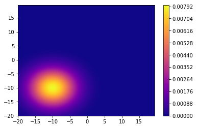
cs = ax2.contourf(X,Y,Z,100, cmap="plasma")
plt.colorbar(cs)
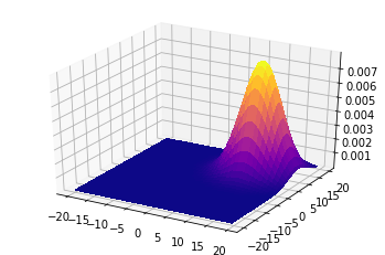
plt.show()fig1では3D描写,fig2では真上から見た濃淡図を出力します。結果は後で示します。
アニメーション描写
from IPython.display import HTML
import matplotlib.animation as animation

def init():
    ax.plot_wireframe(X, Y, Z, rstride=5, cstride=5)
    return fig,

def animate(i):
    ax.view_init(elev=30., azim=3.6*i)
    return fig,

ani = animation.FuncAnimation(fig1, animate, init_func=init, frames=100, interval=100, blit=True)
HTML(ani.to_html5_video())
IPythonのHTMLを利用してアニメーションを出力します。また,matplotlibのanimationを使ってアニメーションを作成します。
結果
平均と分散を変化させて,二次元ガウス分布の性質を考察します。
★望まれる結果
・平均がトンガリの位置を表している
・分散を変化させると縦長,横長に変化する
・共分散を変化させると傾く
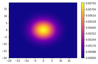
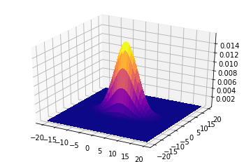
まずは,共分散行列を[[20,0],[0,20]]に固定させます。
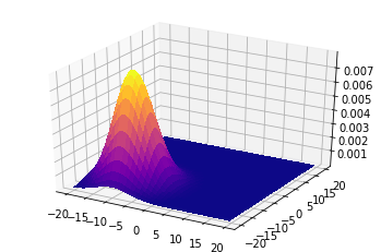
平均=(0, 0)

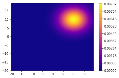
平均=(10, 10)
平均=(-10, -10)
次に,平均を(0, 0)に固定させます。
共分散行列=[[20,0],[0,20]]
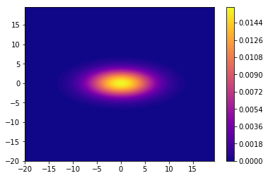
共分散行列=[[20,0],[0,5]]
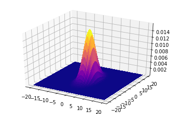
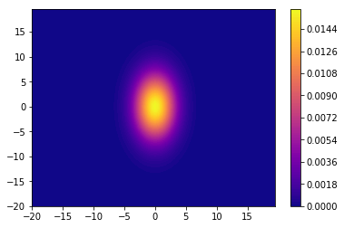
共分散行列=[[5,0],[0,20]]
共分散行列=[[20,10],[10,20]]
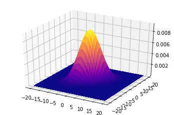
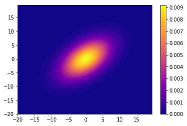
共分散行列=[[20,-10],[-10,20]]
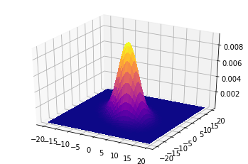
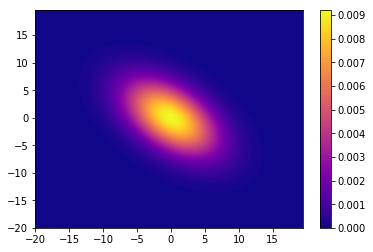
考察
★望まれる結果
・平均がトンガリの位置を表している
・分散を変化させると縦長,横長に変化する
・共分散を変化させると傾く
こちらの予想通りの結果が得られました。特に,共分散行列の定義を理解できているかどうかがポイントになると思います。
もし理論にモヤモヤがあれば

(2026/06/27 15:25:01時点 楽天市場調べ-詳細)
こちらの参考書は,誰もが挫折しかけるPRMLよりも平易に機械学習全般の手法について解説しています。おすすめの1冊になりますので,ぜひお手に取って確認してみてください。