
【超初心者向け】TensorFlowのチュートリアルを読み解く。<その3>


本シリーズでは,ディープラーニングを実装する際に強力な手助けをしてくれる「TensorFlow」についてです。公式チュートリアルを,初心者に向けてかみ砕きながら翻訳していこうと思います。(公式ページはこちらより)
今回はNo.3で,「テキスト解析」編です。その他の記事は,こちらの「TensorFlowの公式チュートリアルを初心者向けに読み解く」をご覧ください。
基本的な流れ
TensolFlowでディープラーニングを実装する流れは,以下のようになります。
●データセットの読み込み
●ネットワークの定義
●最適化アルゴリズムの定義
●学習の実行
●評価の実行
●予測の実行
必要なモジュール等の準備
import tensorflow as tf
from tensorflow import keras
import numpy as np
import matplotlib.pyplot as plt
tensorflowとkerasをインポートしましょう。計算用にnumpy,可視化用にmatplotlib.pyplotもインポートします。
データセットの読み込み
imdb = keras.datasets.imdb
(train_data, train_labels), (test_data, test_labels) = imdb.load_data(num_words=10000)
今回は,映画レビューのデータセットを利用します。教師ラベルは2値で,肯定的か否定的かを表しています。二値分類問題の代表的なデータセットです。具体的には,Internet Movie Databaseから抽出した50,000件の映画レビューを整理した,IMDB dataset を使います。ちなみに,num_wodsという引数は,出現した単語のうち保持する単語数を指定するものです。つまり,あまり出現しない単語は破棄されてしまうというということです。
データセットの概要を確認しましょう。
print("Training entries: {}, labels: {}".format(len(train_data), len(train_labels)))
print(train_data[0])
print(len(train_data[0]), len(train_data[1]))
Training entries: 25000, labels: 25000
[1, 14, 22, 16, 43, 530, 973, 1622, 1385, 65, 458, 4468, 66, 3941, 4, 173, 36, 256, 5, 25, 100, 43, 838, 112, 50, 670, 2, 9, 35, 480, 284, 5, 150, 4, 172, 112, 167, 2, 336, 385, 39, 4, 172, 4536, 1111, 17, 546, 38, 13, 447, 4, 192, 50, 16, 6, 147, 2025, 19, 14, 22, 4, 1920, 4613, 469, 4, 22, 71, 87, 12, 16, 43, 530, 38, 76, 15, 13, 1247, 4, 22, 17, 515, 17, 12, 16, 626, 18, 2, 5, 62, 386, 12, 8, 316, 8, 106, 5, 4, 2223, 5244, 16, 480, 66, 3785, 33, 4, 130, 12, 16, 38, 619, 5, 25, 124, 51, 36, 135, 48, 25, 1415, 33, 6, 22, 12, 215, 28, 77, 52, 5, 14, 407, 16, 82, 2, 8, 4, 107, 117, 5952, 15, 256, 4, 2, 7, 3766, 5, 723, 36, 71, 43, 530, 476, 26, 400, 317, 46, 7, 4, 2, 1029, 13, 104, 88, 4, 381, 15, 297, 98, 32, 2071, 56, 26, 141, 6, 194, 7486, 18, 4, 226, 22, 21, 134, 476, 26, 480, 5, 144, 30, 5535, 18, 51, 36, 28, 224, 92, 25, 104, 4, 226, 65, 16, 38, 1334, 88, 12, 16, 283, 5, 16, 4472, 113, 103, 32, 15, 16, 5345, 19, 178, 32]
(218, 189)訓練用,評価用でそれぞれ25000件のレビューが用意されています。また,用意されたデータは整数値であることが分かります。これは,整数値がある単語に相当するように辞書が定められているからです。そこで,以下ではこの意味不明な整数列をレビューの単語列に変換したいと思います。
word_index = imdb.get_word_index()
word_index = {k:(v+3) for k,v in word_index.items()}
word_index["<PAD>"] = 0
word_index["<START>"] = 1
word_index["<UNK>"] = 2  # unknown
word_index["<UNUSED>"] = 3

reverse_word_index = dict([(value, key) for (key, value) in word_index.items()])

def decode_review(text):
    return ' '.join([reverse_word_index.get(i, '?') for i in text])

decode_review(train_data[0])
"<START> this film was just brilliant casting location scenery story direction everyone's really suited the part they played and you could just imagine being there robert <UNK> is an amazing actor and now the same being director <UNK> father came from the same scottish island as myself so i loved the fact there was a real connection with this film the witty remarks throughout the film were great it was just brilliant so much that i bought the film as soon as it was released for <UNK> and would recommend it to everyone to watch and the fly fishing was amazing really cried at the end it was so sad and you know what they say if you cry at a film it must have been good and this definitely was also <UNK> to the two little boy's that played the <UNK> of norman and paul they were just brilliant children are often left out of the <UNK> list i think because the stars that play them all grown up are such a big profile for the whole film but these children are amazing and should be praised for what they have done don't you think the whole story was so lovely because it was true and was someone's life after all that was shared with us all"元々の単語辞書の最初に新しく4つの単語を登録しています。そして,キーとバリューをひっくり返して,新しく作った単語辞書を使って整数から文章を生成する関数「decode_review」を定義します。実際に,最初のレビューをデコードしてみると,しっかりと文章が生成されていることが確認できます。
さて,訓練データとテストデータを作成しましょう。
train_data = keras.preprocessing.sequence.pad_sequences(train_data,
                                                        value=word_index["<PAD>"],
                                                        padding='post',
                                                        maxlen=256)

test_data = keras.preprocessing.sequence.pad_sequences(test_data,
                                                       value=word_index["<PAD>"],
                                                       padding='post',
                                                       maxlen=256)

x_val = train_data[:10000]
partial_x_train = train_data[10000:]

y_val = train_labels[:10000]
partial_y_train = train_labels[10000:]
今回は,レビューの単語数が異なるため,pad_sequenceというメソッドを利用して長さを揃えます。テストデータは,訓練データの一部を利用します。本来は異なるデータでテストすべきですが,チュートリアルの趣旨上は訓練データを利用して評価してみようということらしいです。
実際に,長さが揃えられていることが分かります。
len(train_data[0]), len(train_data[1])(256, 256)print(train_data[0])[ 1 14 22 16 43 530 973 1622 1385 65 458 4468 66 3941
4 173 36 256 5 25 100 43 838 112 50 670 2 9
35 480 284 5 150 4 172 112 167 2 336 385 39 4
172 4536 1111 17 546 38 13 447 4 192 50 16 6 147
2025 19 14 22 4 1920 4613 469 4 22 71 87 12 16
43 530 38 76 15 13 1247 4 22 17 515 17 12 16
626 18 2 5 62 386 12 8 316 8 106 5 4 2223
5244 16 480 66 3785 33 4 130 12 16 38 619 5 25
124 51 36 135 48 25 1415 33 6 22 12 215 28 77
52 5 14 407 16 82 2 8 4 107 117 5952 15 256
4 2 7 3766 5 723 36 71 43 530 476 26 400 317
46 7 4 2 1029 13 104 88 4 381 15 297 98 32
2071 56 26 141 6 194 7486 18 4 226 22 21 134 476
26 480 5 144 30 5535 18 51 36 28 224 92 25 104
4 226 65 16 38 1334 88 12 16 283 5 16 4472 113
103 32 15 16 5345 19 178 32 0 0 0 0 0 0
0 0 0 0 0 0 0 0 0 0 0 0 0 0
0 0 0 0 0 0 0 0 0 0 0 0 0 0
0 0 0 0]
ネットワークの定義
vocab_size = 10000

model = keras.Sequential()
model.add(keras.layers.Embedding(vocab_size, 16))
model.add(keras.layers.GlobalAveragePooling1D())
model.add(keras.layers.Dense(16, activation=tf.nn.relu))
model.add(keras.layers.Dense(1, activation=tf.nn.sigmoid))

model.summary()
Model: "sequential"
_________________________________________________________________
Layer (type) Output Shape Param #
=================================================================
embedding (Embedding) (None, None, 16) 160000
_________________________________________________________________
global_average_pooling1d (Gl (None, 16) 0
_________________________________________________________________
dense (Dense) (None, 16) 272
_________________________________________________________________
dense_1 (Dense) (None, 1) 17
=================================================================
Total params: 160,289
Trainable params: 160,289
Non-trainable params: 0
_________________________________________________________________最初に,kerasのsequentialモデルのインスタンスを生成しています。sequentialモデルは深層学習の中でも最も基本的なモデルで,層を単純に重ねるだけのモデルを指しています。
次に,作成したインスタンスに2つの層を追加しています。1層目は次元を16次元まで落とEembedding層です。2層目は圧縮データの次元方向に平均を取るプーリング層です。3層目はシンプルな全結合層で,4層目はシグモイドを取る出力層です。
最適化アルゴリズムの定義
model.compile(optimizer=tf.keras.optimizers.Adam(),
              loss='binary_crossentropy',
              metrics=['accuracy'])
モデルインスタンスのcompileメソッドによって,学習に利用する最適化アルゴリズムの詳細を設定できます。optimizer引数でAdamを指定しています。誤差関数はクロスエントロピー,評価関数はaccuracyを設定しています。
学習の実行
history = model.fit(partial_x_train,
                    partial_y_train,
                    epochs=40,
                    batch_size=512,
                    validation_data=(x_val, y_val),
                    verbose=1)
modelインスタンスのfitメソッドで学習を実行しています。学習とは,ネットワークの重みを学習データに適合(fit)させることを指しています。epochsはバッチサイズの学習を何回繰り返すかを表しています。validation_dataは,評価に利用するデータセットの設定です。verboseは学習中に経過を出力するかのオプションです。
historyという変数に代入することで,以下のように学習過程を視覚化することができます。
#Accuracy
plt.plot(history.history['acc'])
plt.plot(history.history['val_acc'])
plt.title('model accuracy')
plt.ylabel('accuracy')
plt.xlabel('epoch')
plt.legend(['train', 'test'], loc='upper left')
plt.show()
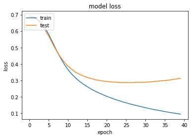
#loss
plt.plot(history.history['loss'])
plt.plot(history.history['val_loss'])
plt.title('model loss')
plt.ylabel('loss')
plt.xlabel('epoch')
plt.legend(['train', 'test'], loc='upper left')
plt.show()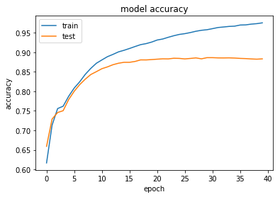
評価の実行
score = model.evaluate(x_val, y_val)
print('Test loss:', score[0])
print('Test accuracy:', score[1])
Test loss: 0.31101081615686416
Test accuracy: 0.8833上でも評価は行っていますが,改めてscoreに代入します。出力から最終的なlossとaccuracyを読み取れます。約88%の精度が出ました。
予測の実行
今回は行っておりません。